
In this note, I will progressively explain some basics of antenna theory and will present the results of antenna modeling. I had already used a few terms (directivity, impedance), which I had not introduced yet. So I think it is a good time for this.
Lets  will be normalized on peak value radiation pattern. The directivity is:

On the pictures below, I had shown a few radiation patterns simulated for my antenna in 4nec2 and CST. In horizontal and vertical plates they are slightly different. The narrower the radiation pattern, the higher is directivity
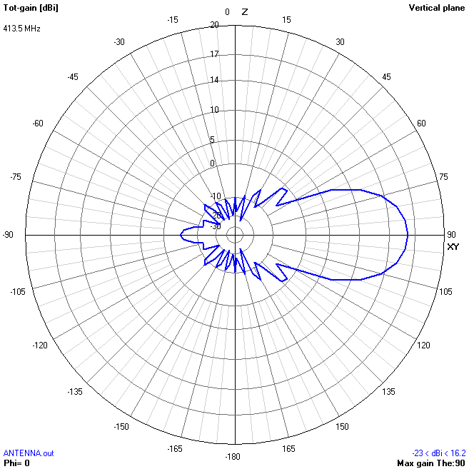
Radiation pattern in the vertical plane. 4nec2 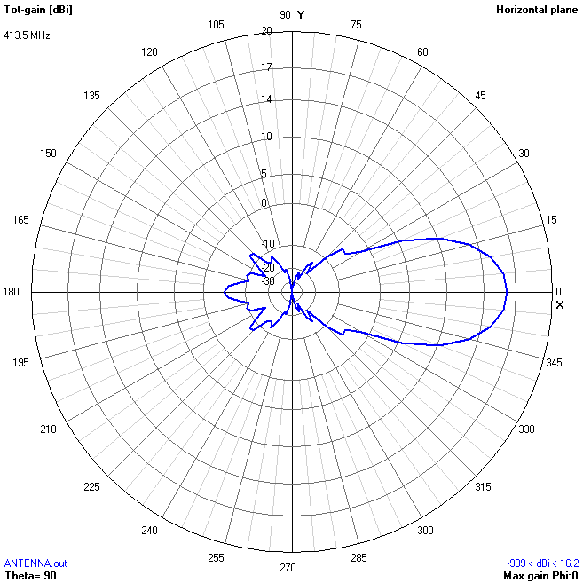
Radiation pattern in the horizontal plane. 4nec2 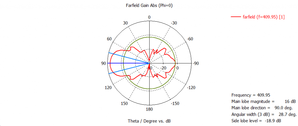
Radiation pattern in the horizontal plane. CST
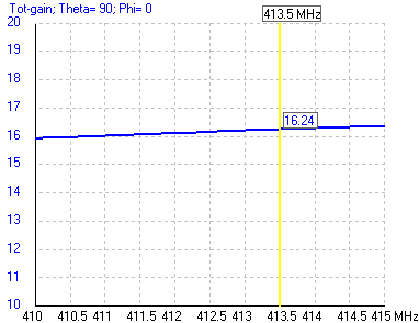
The higher the directivity, the higher is antenna gain:

where  is radiation efficiency.
  . The term radiation efficiency appears due to the nonzero resistance of antenna materials (metal and dielectric). So some part of the input power goes on radiation and some of it goes on heating of the antenna elements. This is why antenna made with copper or with silver coating are more efficient than antennas made of aluminum or steel. The losses
  due to matching problems of antenna and transmission line goes into total efficiency of antenna
The effective area of the antenna:

For example, for an antenna on 410 MHz with 16 dB gain have an effective area of  .
.
To send (or receive) 100% of power in antenna, we need to match the impedance of the transmission line  and antenna impedance
  . If these two impedances are badly matched, we would have reflection of part of the power with a coefficient of reflection:

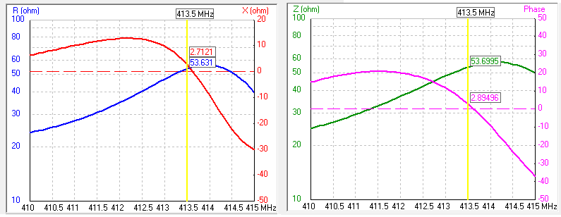
Simulated in 4nec2 the impedance of antenna
You can check here how to derive this coefficient. It is a complex value. The absolute value of it is  parameter. This value depends on the frequency and has a minimum on the working frequency of the antenna. The ration of the working frequency to the antenna bandwidth is quality factor Q.
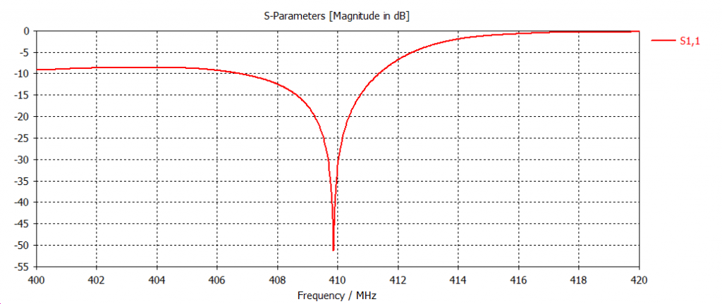
Calculated in CST parameter S11 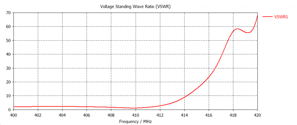
Calculated in CST parameter VSWR
However, in practice is more used SWR (standing wave ratio) value because it is easier to measure. Depending on how you measure it (on voltage or current), people distinguish VSWR (more used) and ISWR. The definition of SWR is:

When you tune the antenna, you try to minimize this value. To measure SWR there are two main schemas: one on a directional coupler and the other on a resistive bridge.
Schema with directional coupler
The circuit with directional coupler is popular on low frequencies, but on UHF it doesn't work die to maximum working frequency of the ferrite in current transformer. The modification of this schema with a coupler made on PCB alllows to measure SWR up to 145 and 430 MHz. You can learn more about this here and here. The scale of the sensor is nonlinear because the measured value is inversely proportional to the desired.
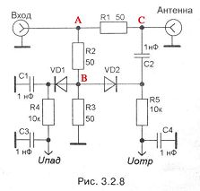
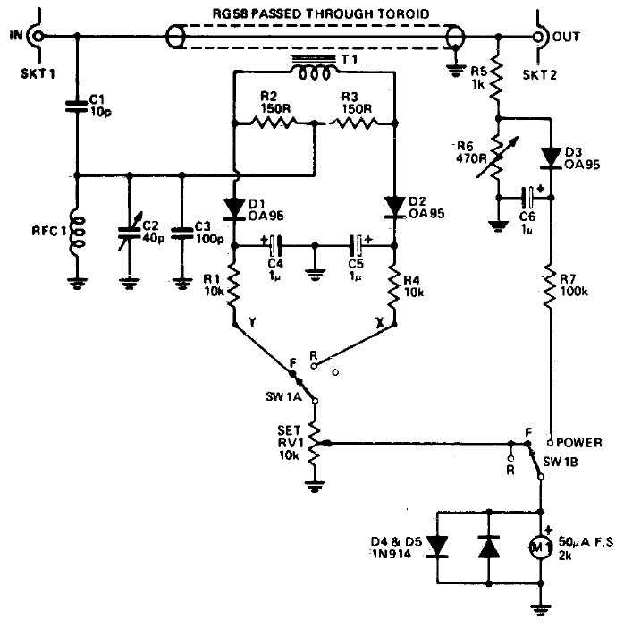
Bridge schema to measure SWR (Honcharenko)
On the higher frequencies more popular is bridge schema. However, the true values are measured by it only in case of zero reactance. Some antenna analyzers combine the measurements of amplitude with measurements of phase. Why we need to measure the phase and how we can measure complex impedance is well described here.
I would like also to introduce a Smith diagram (chart). In old good times, when the computational resources were limited, for manipulation with complex impedance people uses Smith chart. Nowadays it is not so in demand, but I advise to have a look at this simple and genial idea at least for general education. Simulated impedance on Smith chart you can see on the top of the note.
I would like to show once again Transmission line impedance equation (Pozar, Microwave engineering):

when tangent is equal to  , we have a half-wave transformer (we already had discussed this). But when tangent equal to , the impedance of line doesn't matter at all

that's mean that on the output of the line we see clear impedance of the antenna. we have this situation only when the cable length is equal to the integer part of half-wave (multiplied by shortening coefficient of the cable).
That's all for today. The next note will be more practical.