
In this project, I aim to detect only one pulsar - B0329 + 54. It is the most powerful radio pulsar in the Northern Hemisphere. It is located in the constellation Camelopardalis ( Girafe ) and should be easy to find.
Data from ATNF Pulsar Catalogue
Name B0329+54
PSRJ J0332+5434
Right Ascension 03:32:59.368
Declination +54:34:43.57
Period of pulse 0.714519699726 s
Dispersion measure 26.7641
Width of the pulse measured between 50% power points of the pulse 6.6 (ms)
Width of the pulse measured between 10% power points of the pulse 31.4 ms
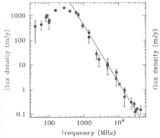
S400 - flux density at 400 MHz is 1500 mJy
S1400 - flux density at 1400 MHz is 203 mJy
 , where
  is the spectral index (-1.8 on average)
The pulsar emission spectrum is wide, however, in most cases, the pulsar is monitored at two frequencies: 400MHz and/or 1400MHz.
I chose 400 MHz because there are some advantages to work at low frequency:
- The signal is stronger. The scintillation time is shorter (will be discussed later)
- The electronics are cheaper
- The permissible errors in antenna fabrication are higher.
However, the dispersion of the signal is larger (the pulse spreads over a period and becomes more difficult to detect). Also, the EM noise is larger and you may need to install a telescope far from the city, which requires a telescope to be portable.
When the signal travels through the interstellar space, the signal disperses and so the longer waves arrive with a delay:

DM is a measure of the dispersion and the frequency is in MHz. Since the path from each of the pulsars to the Earth is unique, so the measure of dispersion is unique for each pulsar too. The greater the dispersion, the more blurred the pulse over the period will be. However, there are a few techniques for signal dedispersion.
The signal travels not just through the interstellar vacuum but through the turbulent interstellar medium. This leads to constructive/destructive interference of the pulse wavefront. Let's consider a simple case when we have the diffraction on the circular aperture: when the light passes through it, on the screen you will see a beautiful Airi disk. Now instead of the aperture with clear borders, there is an interstellar medium that distorts the wavefront of the signal and on the antenna of the radio telescope instead of a beautifully clear picture, there is a map of light and dark spots. And as this interstellar environment (space weather) moves, this pattern changes too. It is somehow similar to the terrestrial observations through the earth's atmosphere in the optical range.
As a result, the pulse-to-pulse amplitude is different (as for an example look at the first video on the page). This effect is called scintillation. The pulsar signal may disappear for a while, but this is a characteristic time for which it disappears and appears is lower at lower frequencies, so the results of the measurement will be more repeatable from one observation to another.
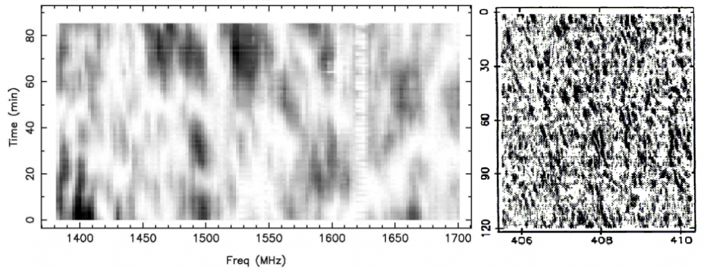
B0329 + 54 pulsar scintillation at 408 MHz and 1.5 GHz for 1.5-2 hours duration
The polarization of the pulsar radiation should also be taken into account. For each pulsar, the polarization is different. Hopefully, for B0329 + 54 the radiation is relatively linearly polarized. Traveling through the interstellar medium, the Faraday polarization vector "rotates in space". Therefore, it is unlikely to orient the antenna to the "correct" position, but it is better to wait until after some time it returns itself, although the choice of "good" orientation of the telescope can reduce the influence of local radio interference.
The choice of the bandwidth is with the catch. According to the equation, the larger the bandwidth is the better, but there are two factors that do not allow you to set an infinite bandwidth:
- The maximum bandwidth of the receiver. If you use the SDR receiver, then its maximum band can be checked here. In Chinese RTL-SDR, the maximum bandwidth is 2.4-2.8 MHz.
- The measure of dispersion. The maximum band is calculated when the dispersion delay is half the pulse width at half height (HWHM).
For B0329 + 54 the maximum bandwidth is limited by dispersion and it is 1MHz.
Therefore, we have: The flux density for B0329 + 54 at 400 MHz is 1.5 Jy, the dispersion measure = 27. If we take S / N = 4 and  , the observation time of 1 hour and bandwidth of 1 MHz, so we can derive minimum gain of the antenna from radiometer equation:

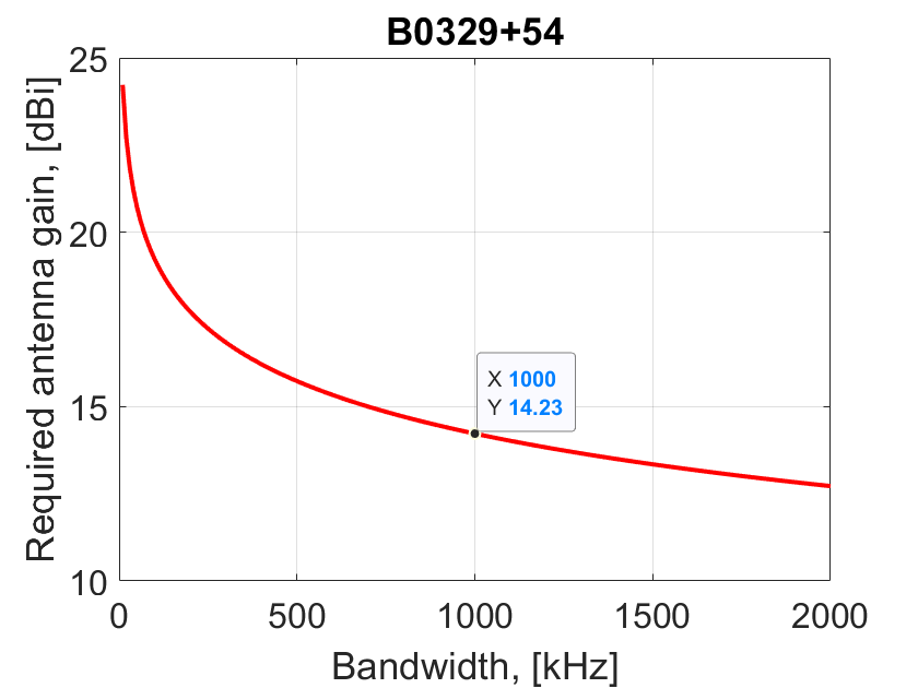
The dependence of the antenna gain  in the radiometric equation on the bandwidth:
%MATLAB script to calculate required gain
clear all; close all; clc
SN=4;
S=1.5e-26;
Tsys=100;
t=3600;
lambda=3e+8/4e+8;
df=1e+4:1e+4:2e+6;
np=1;
kb=1.38e-23;
beta=1;
P=0.714519;
W=6.6e-3;

A=beta*2*kb*SN*Tsys*sqrt(W/(P-W))./(sqrt(np*t*df))/S;

G=4*pi*A/lambda^2;

figure
plot(df*1e-3,10*log10(G),'r','linew',2)
grid on
set(gca,'fontsize',16)
xlabel('Bandwidth, [kHz]')
ylabel('Required antenna gain, [dBi]')
title('B0329+54')
so we get that the minimum gain for the 1MHz bandwidth is 14 dB. Of course, this value is theoretically minimal and the actual gain of the antenna should be at least 14dB, or even 17 or 19dB.
In fact, the radiometric equation requires an improvement:

That is, the noise of high-frequency interference (radio, television, communications, equipment) is significant. It is difficult to place the antenna far from interference and this is a significant problem for amateur radio astronomers with small antennas. However, observation times and hours are usually unlimited. Radio surveillance at night is cleaner, due to fewer devices in use.
Noise from the ground, buildings, trees are added through the sidelobes of the antenna sensitivity pattern, which also does not help in observations.
I highly recommend reading this link. Much of the info here and in the previous notes were taken from there.