
Let us consider a source of unpolarized flux density  . This flux is collected by a telescope with an effective area of
  , where
  is the geometric area of the telescope and
  is the efficiency of the telescope. Since the contribution of each of the polarization is half in the total flux, so the power density [
 ] on the receiver is a simple product
On the other hand, let us consider the antenna as a simple resistive load. The received flux "heats" this load to temperature  . The chaotic thermal motion of electrons ( Johnson-Nyquist noise) in this load causes an alternating voltage in this scheme which is measured. As the thermal motion noise has a power density of
  (
( is the Boltzmann constant), so flux can be replaced by temperature:

where G (gain) is gain of the antenna. To derive this,  was used. The gain here is not in dB or times but in units of K/Jy. The example of gain for two telescopes:
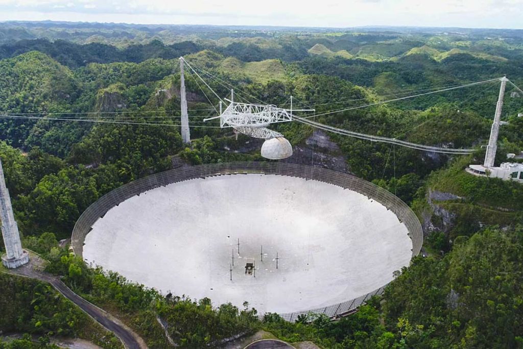
Arecibo G=20 K/Jy. The biggest radiotelecope in free world 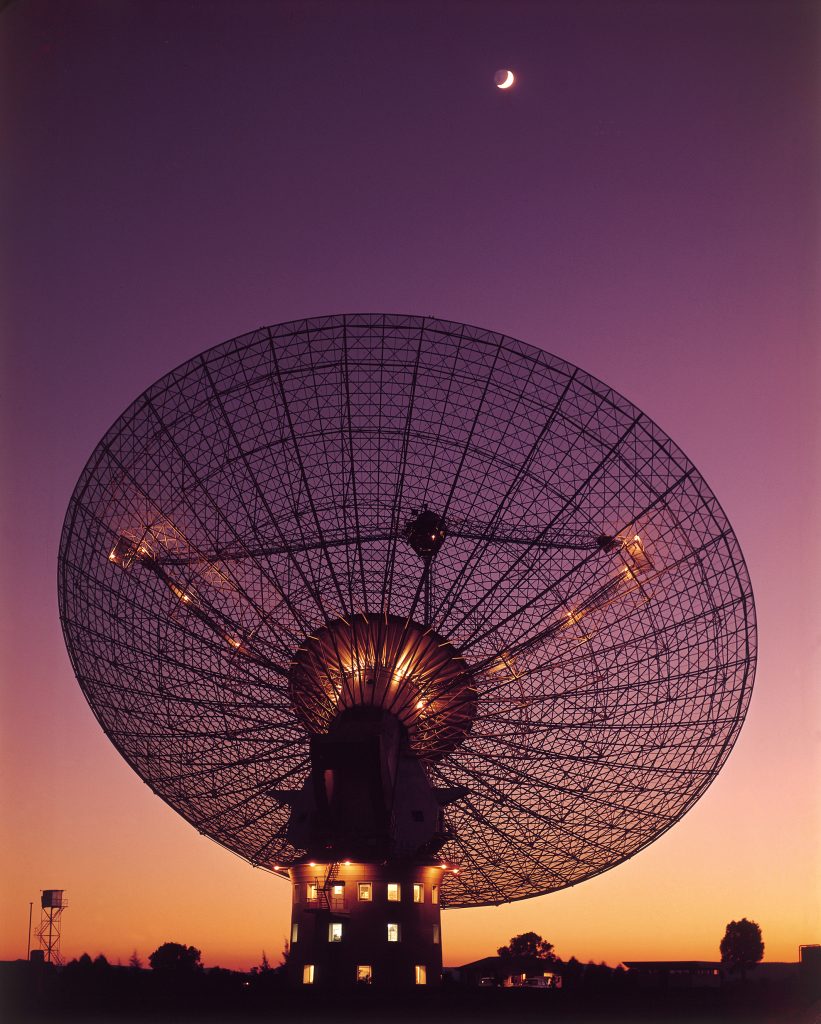
Parkes G=0.64 K/Jy. This telescope receives the TV signal during Apollo 11 mission.
The usage of temperature units for flux is much more convenient in practice. However, even before the receival, the antenna is already heated to some temperature of the receiving system  . This temperature is basically noise:

where  is receiver noise (approximately 20 K for the cooled systems),
  is (spillover noise) antenna noise (10 K),
  arises from the radiation of the Earth's atmosphere, and
  is the background radiation of the sky (CMB, synchrotron radiation in the Galaxy plane) and depends on the point and frequency of observation (10-30K, in the center of the Galaxy 800K).
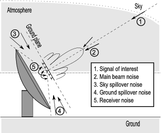
Illustration to explain the various noise contributions 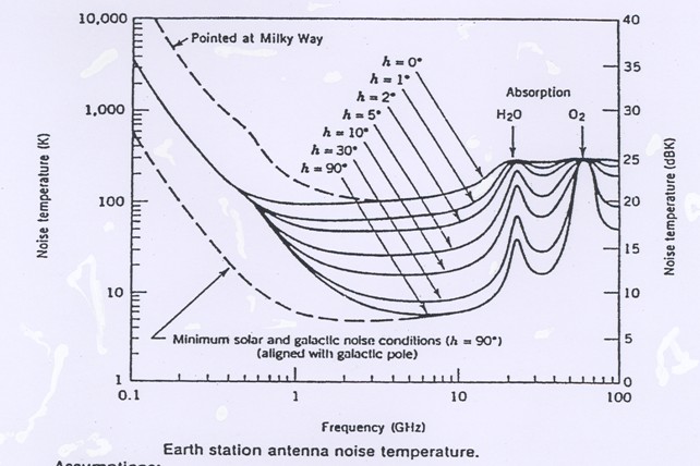
Sky noise
Radiometer equation
It is logic to assume that the signal can be detected if it is stronger than the noise fluctuations in the receiving system. The RMS value of the fluctuations is:

where  is the bandwidth of the receiver,
  is the duration of the reception, and
  is 1 if we receive in one polarization or 2 if in two. This formula is called the radiometer equation and is the basis of the most radio astronomical systems sensitivity calculations. Let's derive the radiometer equation for the sensitivity to receive pulse signals.
Let's we have a pulse with a period of  , a width of
  , and a peak amplitude of
  , which sits above the noise of . The noise fluctuations in this case are sums of two parts: in the moment when pulse is present
  and when there is no pulse
  :
:

It's ok to assume that  , so we have:

where  is the observation time.
Okay. Now signal / noise is  by definition, then

If you now go back to the density of the flux, the average of the period will be:


You can already use this equation. Sometimes there is a need to determine the minimum flux density that a radio telescope can detect, and then an additional correction factor  is introduced for the non-perfection of the system.

Oddities arise from signal digitization and other effects. Usually is a little more than one.
So the smaller the  , the weaker signals of the pulsars can be observed. It can also be seen from the equation that it is easier to observe pulsars with a narrow pulse width . The quality of the data depends also on the observation time
  and the bandwidth of the receiver. However, this two are under root, so an increase of the observation time by four times will only improve the data by a factor two. The increase in the antenna gain
  or to reduce the noise is more efficient as they are in linear proportionality. To be scientifically clear, a high signal/noise value of
  is required to reliably confirm the pulsar signal. Professional astronomers use
  , but for amateurs
  is enough.
I recommend to read the "Handbook of pulsar astronomy" of Lorimer and Framer. This note is basically one of the appendixes.